Solutions - Exercices sur la dimension - 01

Solutions détaillées de neuf exercices sur la notion de dimension en algèbre linéaire (fiche 01).
Cliquer ici pour accéder aux énoncés.

Divers éléments théoriques sont disponibles dans cet article.

Selon la formule de Grassmann :

$\dim\left(F\cap G\right)=\dim\left(F\right)+\dim\left(G\right)-\dim\left(F+G\right)$

or $\dim\left(F\right)=a,$ $\dim\left(G\right)=b$ et $\dim\left(F+G\right)\leqslant a+b-1.$

Il s’ensuit que :

$\dim\left(F\cap G\right)\geqslant a+b-\left(a+b-1\right)=1$

Ceci prouve l’existence d’un vecteur non nul dans $F\cap G$ (ou, ce qui revient au même, d’une droite vectorielle incluse dans $F\cap G).$

Si $f$ est une homothétie, il est évident que $C_{f}=\mathcal{L}\left(E\right)$ et donc (vu que $\dim\left(E\right)=2)$ :

$\boxed{\dim\left(C_{f}\right)=4}$

Supposons désormais que $f$ n’est pas une homothétie.

D’après la caractérisation des homothéties, il existe un vecteur $e\in E$ tel que $\beta=\left(e,f\left(e\right)\right)$ soit libre. Cette famille est donc une base de $E.$

Considérons l’application :

$\boxed{\varphi:C_{f}\rightarrow E,\thinspace g\mapsto g\left(e\right)}$

➢➢ La linéarité de $\varphi$ est évidente.

➢➢ Injectivité de $\varphi$ :

Si $g\in\ker\left(\varphi\right)$ alors $g\left(e\right)=0_{E}$ donc $g\left(f\left(e\right)\right)=f\left(g\left(e\right)\right)=f\left(0_{E}\right)=0_{E}.$ Ceci entraîne que $g$ est l’endomorphisme nul (une application linéaire qui s’annule sur une base est l’application nulle).

➢➢ Surjectivité de $\varphi$ :

Soit $x\in E.$ Décomposons $x$ dans la base $\beta,$ sous la forme :

$x=\lambda\thinspace e+\mu\thinspace f\left(e\right)$

alors :

$x=\left(\lambda\thinspace id_{E}+\mu\thinspace f\right)\left(e\right)$

et comme $\lambda\thinspace id_{E}+\mu\thinspace f\in C_{f},$ ceci prouve que $\varphi\left(\lambda\thinspace id_{E}+\mu\thinspace f\right)=x.$

En définitive, $\varphi$ est un isomorphisme. Il en résulte que :

$\boxed{\dim\left(C_{f}\right)=2}$

Considérons la base canonique $\left(E_{p,q}\right)_{1\leqslant p,q\leqslant n}$ de $\mathcal{M}_{n}\left(\mathbb{K}\right)$ et translatons-la de $I_{n}$ .

Ceci signifie simplement qu’on ajoute la matrice unité à chaque matrice élémentaire pour fabriquer une nouvelle famille de $n^{2}$ matrices.

Prouvons que la famille $\left(I_{n}+E_{p,q}\right)_{1\leqslant p,q\leqslant n}$ est une base de $\mathcal{M}_{n}\left(\mathbb{K}\right).$

Notons $F_{p,q}=I_{n}+E_{p,q};$ si $M\in\mathcal{M}_{n}\left(\mathbb{K}\right)$ alors :

$\begin{eqnarray*} M & = & \sum_{1\leqslant p,q\leqslant n}m_{p,q}E_{p,q}\\& = & \sum_{1\leqslant p,q\leqslant n}m_{p,q}\left(F_{p,q}-I_{n}\right)\\& = & \left(\sum_{1\leqslant p,q\leqslant n}m_{p,q}F_{p,q}\right)-\mu I_{n}\end{eqnarray*}$

avec :

$\mu=\sum_{1\leqslant p,q\leqslant n}m_{p,q}$

Or :

$\sum_{p=1}^{n}F_{p,p}=\left(n+1\right)I_{n}$

et donc :

$M=\left(\sum_{1\leqslant p,q\leqslant n}m_{p,q}F_{p,q}\right)-\frac{\mu}{n+1}\sum_{p=1}^{n}F_{p,p}$

ce qui prouve que $\left(F_{p,q}\right)_{1\leqslant p,q\leqslant n}$ est génératrice de $\mathcal{M}_{n}\left(\mathbb{K}\right).$

Comme cette famille comporte $n^{2}$ matrices, c’est bien une base de $\mathcal{M}_{n}\left(\mathbb{K}\right).$

Enfin, on constate que les $F_{p,q}$ sont toutes inversibles, puisque ce sont des matrices triangulaires (voire diagonales pour certaines d’entre-elles) dont les termes diagonaux sont tous nuls.

Considérons l’application $\theta$ définie par :

$\begin{eqnarray*} E_{n} & \rightarrow & \mathbb{R}^{n+1}\\ f & \mapsto & \left(f\left(0\right),f\left(\frac{1}{n}\right),\cdots,f\left(\frac{n-1}{n}\right),f\left(1\right)\right) \end{eqnarray*}$

Il est clair que $f$ est linéaire.

Si $f\in\ker\left(\theta\right),$ alors $f\left(\frac{k}{n}\right)=f\left(\frac{k+1}{n}\right)=0$ pour tout $k\in\left\llbracket 0,n-1\right\rrbracket .$ Et comme la restriction de $f$ à $\left[\frac{k}{n},\frac{k+1}{n}\right]$ est affine, elle est nulle et donc $f=0.$ Ainsi $\theta$ est injective.

Etant donné $j\in\left\llbracket 1,n-1\right\rrbracket ,$ considérons l’application $f_{j}$ définie par :

$\boxed{\forall x\in\left[0,1\right],\:f_{j}\left(x\right)=\left\{ \begin{array}{ccc}nx-j+1 & \textrm{si} & x\in\left[\frac{j-1}{n},\frac{j}{n}\right]\\\\-nx+j+1 & \textrm{si} & x\in\left[\frac{j}{n},\frac{j+1}{n}\right]\\\\0 & \textrm{sinon}\end{array}\right.}$

Posons de plus :

$\boxed{f_{0}\left(x\right)=\left\{ \begin{array}{ccc}-nx+1 & \textrm{si} & x\in\left[0,\frac{1}{n}\right]\\0 & \textrm{sinon}\end{array}\right.}$

$\boxed{f_{n}\left(x\right)=\left\{ \begin{array}{ccc}nx-n+1 & \textrm{si} & \textrm{x}\in\left[\frac{n-1}{n},1\right]\\0 & \textrm{sinon}\end{array}\right.}$

On observe que $\forall j\in\left\llbracket 0,n\right\rrbracket ,\,f_{j}\in E_{n}$ et que $f_{j}\left(\frac{k}{n}\right)=\delta_{j,k}.$

Soit alors $\left(b_{0},\cdots,b_{n}\right)\in\mathbb{R}^{n+1};$ l’application

$f=\sum_{j=0}^{n}\,b_{j}\,f_{j}$

appartient à $E_{n}$ et vérifie :

$\forall k\in\left\llbracket 0,n\right\rrbracket ,\,f\left(\frac{k}{n}\right)=b_{k}$

Ceci montre la surjectivité de $\theta.$ Finalement, $\theta$ est un isomorphisme et donc :

$\boxed{\dim\left(E_{n}\right)=n+1}$

Notons $A$ une primitive de $u$ (on rappelle que toute application continue d’un intervalle $I\subset\mathbb{R}$ dans $\mathbb{R}$ admet des primitives). Soit $f:I\rightarrow\mathbb{R}$ dérivable et soit :

$F:I\rightarrow\mathbb{R},\thinspace x\mapsto f\left(x\right)\thinspace e^{-A\left(x\right)}$

Alors $F$ est dérivable et :

$\forall x\in I,\thinspace F'\left(x\right)=\left(f'\left(x\right)-u\left(x\right)\thinspace f\left(x\right)\right)\thinspace e^{-A\left(x\right)}$

Par conséquent :

$\boxed{f\in E\Leftrightarrow F\text{ est constante}}$

Ainsi, $E$ est la droite vectorielle engendrée par $x\mapsto e^{A\left(x\right)}$ et, en particulier : $\dim\left(E\right)=1.$

Remarque

Ce qui précède est fondamental :

Si $u:I\rightarrow\mathbb{R}$ est continue, l’espace des solutions sur $I$ de l’équation différentielle

$\boxed{y'=u\left(x\right)\thinspace y}$

est une droite vectorielle.

Considérons maintenant l’équation différentielle :

$x\left(x-1\right)\thinspace y'=2\left(2x-1\right)\thinspace y$

Pour trouver ses solutions sur $\mathbb{R},$ on cherche d’abord ses solutions l’un des trois intervalles suivants :

$I_{0}=\left]-\infty,0\right[,\quad I_{1}=\left]0,1\right[,\quad I_{2}=\left]1,+\infty\right[$

sur chacun desquels la quantité $x\left(x-1\right)$ ne s’annule pas.

Ceci permet de se ramener à l’équation différentielle $y'=u\left(x\right)\thinspace y$ avec :

$u\left(x\right)=\frac{2\left(2x-1\right)}{x\left(x-1\right)}$

Si $k\in\left\{0,1,2\right\} ,$ alors une primitive sur $I_{k}$ de $u$ est donnée par :

$x\mapsto2\ln\left|x^{2}-x\right|$

Les solutions sur $I_{k}$ sont donc les :

$x\mapsto\lambda\thinspace\left(x^{2}-x\right)^{2}$

Par conséquent, si $f$ est une solution sur $\mathbb{R},$ alors il existe $\left(\lambda_{0},\lambda_{1},\lambda_{2}\right)\in\mathbb{R}^{3}$ tel que $f$ soit définie par :

$\boxed{x\mapsto\left\{\begin{array}{cc}\lambda_{0}\left(x^{2}-x\right)^{2} & \text{si }x\leqslant0\\\lambda_{1}\left(x^{2}-x\right)^{2} & \text{si }0<x\leqslant1\\\lambda_{2}\left(x^{2}-x\right)^{2} & \text{si }x>1\end{array}\right.}$

Réciproquement, l’application ainsi définie est dérivable quel que soit $\left(\lambda_{0},\lambda_{1},\lambda_{2}\right)\in\mathbb{R}^{3}$ et c’est donc une solution sur $\mathbb{R}.$

En conclusion :

$\boxed{\dim\left(F\right)=3}$

Une base de $F$ est $\left(\varphi_{0},\varphi_{1},\varphi_{2}\right)$ avec :

$\boxed{\varphi_{0}:\mathbb{R}\rightarrow\mathbb{R},\thinspace x\mapsto\left\{ \begin{array}{cc}\left(x^{2}-x\right)^{2} & \text{si }x<0\\0 & \text{sinon} \end{array}\right.}$

$\boxed{\varphi_{1}:\mathbb{R}\rightarrow\mathbb{R},\thinspace x\mapsto\left\{ \begin{array}{cc} \left(x^{2}-x\right)^{2} & \text{si }0<x<1\\0 & \text{sinon}\end{array}\right.}$

$\boxed{\varphi_{2}:\mathbb{R}\rightarrow\mathbb{R},\thinspace x\mapsto\left\{ \begin{array}{cc} \left(x^{2}-x\right)^{2} & \text{si }x>1\\0 & \text{sinon}\end{array}\right.}$

Illustration dynamique

L’illustration dynamique ci-dessous permet de visualiser les solutions.

Les trois sliders contrôlent respectivement les coefficients $\lambda_{0},$ $\lambda_{1}$ et $\lambda_{2}.$

En positionnant deux de ces trois coefficients à 0, on peut voir le graphe d’une solution proportionnelle à l’une des $\varphi_{i}.$

Translater le système de coordonnées en pressant SHIFT →↑↓←.

Zoomer / dézoomer en utilisant les touches P / M.

Notons $\tilde{f}$ la restriction de $f$ à $\mbox{Im}\left(g\right).$ Son noyau et son image sont respectivement :

$\ker\left(\tilde{f}\right)=\ker\left(f\right)\cap\mbox{Im}\left(g\right)$

$\mbox{Im}\left(\tilde{f}\right)=\mbox{Im}\left(f\circ g\right)$

Le théorème du rang appliqué à $\tilde{f}$ donne :

( $\star$ ) $\mbox{rg}\left(g\right)=\dim\left(\ker\left(f\right)\cap\mbox{Im}\left(g\right)\right)+\mbox{rg}\left(f\circ g\right)$

Toujours d’après le théorème du rang :

$\left\{ \begin{array}{ccc}\mbox{rg}\left(g\right) & = & n-\dim\left(\ker\left(g\right)\right)\\\\\mbox{rg}\left(f\circ g\right) & = & n-\dim\left(\ker\left(f\circ g\right)\right)\end{array}\right.$

d’où, en reportant dans $\left(\star\right)$ :

$\dim\left(\ker\left(f\circ g\right)\right)=\dim\left(\ker\left(f\right)\cap\mbox{Im}\left(g\right)\right)+\dim\left(\ker\left(g\right)\right)$

Comme $\ker\left(f\right)\cap\mbox{Im}\left(g\right)\subset\ker\left(f\right),$ on voit que :

( $\heartsuit$ ) $\boxed{\dim\left(\ker\left(f\circ g\right)\right)\leqslant\dim\left(\ker\left(f\right)\right)+\dim\left(\ker\left(g\right)\right)}$

L’égalité dans $\left(\heartsuit\right)$ se produit lorsque l’inclusion $\ker\left(f\right)\cap\mbox{Im}\left(g\right)\subset\ker\left(f\right)$ est une égalité, c’est-à-dire lorsque $\ker\left(f\right)\subset\text{Im}\left(g\right).$

Passons à la seconde inégalité.

L’inclusion évidente $\ker\left(g\right)\subset\ker\left(f\circ g\right)$ donne, en passant aux dimensions :

$\dim\left(\ker\left(g\right)\right)\leqslant\dim\left(\ker\left(f\circ g\right)\right)$

Par ailleurs, l’inclusion évidente $\text{Im}\left(f\circ g\right)\subset\text{Im}\left(f\right)$ donne $\text{rg}\left(f\circ g\right)\leqslant\text{rg}\left(f\right)$ et donc, via la formule du rang :

$\dim\left(\ker\left(f\right)\right)\leqslant\dim\left(\ker\left(f\circ g\right)\right)$

Ainsi :

( $\diamondsuit$ ) $\boxed{\max\left\{ \dim\left(\ker\left(f\right)\right),\thinspace\dim\left(\ker\left(g\right)\right)\right\} \leqslant\dim\left(\ker\left(f\circ g\right)\right)}$

L’égalité dans $\left(\diamondsuit\right)$ se produit lorsque $\ker\left(f\circ g\right)=\ker\left(g\right)$ ou $\text{Im}\left(f\circ g\right)=\text{Im}\left(f\right).$

On peut compléter la famille libre $\left(v_{1},\cdots,v_{r}\right)$ en une base

$B=\left(v_{1},\cdots,v_{r},v_{r+1},\cdots,v_{n}\right)$

de $E.$ Notons :

$B^{\star}=\left(v_{1}^{\star},\cdots,v_{r}^{\star},v_{r+1}^{\star},\cdots,v_{n}^{\star}\right)$

sa base duale. Rappelons que, pour tout $i\in\left\llbracket 1,n\right\rrbracket ,$ $v_{i}^{\star}$ désigne la forme linéaire définie par :

$\boxed{\forall j\in\left\llbracket 1,n\right\rrbracket ,\thinspace v_{i}^{\star}\left(v_{j}\right)=\delta_{i,j}}$

et que $B^{\star}$ est une base de l’espace $\mathcal{L}\left(E,\mathbb{K}\right)$ des formes linéaires sur $E.$

L’expression de toute forme linéaire $\varphi$ dans la base $B^{\star}$ est :

$\varphi=\sum_{i=1}^{n}\varphi\left(v_{i}\right)\thinspace v_{i}^{\star}$

Il en résulte que si l’on pose, pour tout $i\in\left\llbracket 1,r\right\rrbracket$ :

$F_{i}=\left\{ \varphi\in\mathcal{L}\left(E,\mathbb{K}\right);\thinspace\varphi\left(v_{i}\right)=0\right\}$

alors :

$\boxed{\bigcap_{i=1}^{r}F_{i}=\text{vect}\left(v_{r+1}^{\star},\cdots,v_{n}^{\star}\right)}$

et donc :

$\boxed{\dim\left(\bigcap_{i=1}^{r}F_{i}\right)=n-r}$

Il semble que le plus clair consiste à raisonner matriciellement. Notons :

$a=\dim\left(A\right),$
$b=\dim\left(B\right),$
$\beta=\left(e_{1},\cdots,e_{a}\right)$ une base de $A,$ complétée en une base $\left(e_{1},\cdots,e_{n}\right)$ de $E,$
$\gamma=\left(f_{1},\cdots,f_{b}\right)$ une base de $B,$ complétée en une base $\left(f_{1},\cdots,f_{n}\right)$ de $E,$
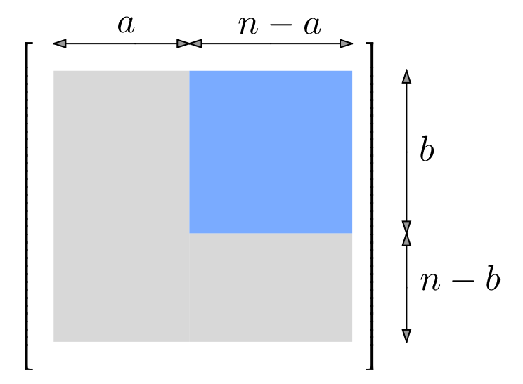
$W$ le sous-espace vectoriel de $\mathcal{M}_{n}\left(\mathbb{K}\right)$ constitué des matrices dont les termes situés en ligne $i$ et colonne $j$ avec $i>b$ ou $j\leqslant a$ sont tous nuls.

Dans l’illustration ci-dessous, tous les termes de la zone grisée sont nuls, les autres (zone bleutée) sont arbitraires :

En associant à tout $f\in V$ sa matrice relativement aux bases $\beta$ et $\gamma$ , on définit une application linéaire de $V$ vers $W.$ Cette application est bijective car une application linéaire est entièrement déterminée par la donnée des images des vecteurs d’une base. En outre, si $\left(E_{p,q}\right)_{1\leqslant p,q\leqslant n}$ désigne la base canonique de $\mathcal{M}_{n}\left(\mathbb{K}\right),$ alors la sous famille $\left(E_{p,q}\right)_{{1\leqslant p\leqslant b\atop a+1\leqslant q\leqslant n}}$ est une base de $W,$ et donc $\dim\left(W\right)=\left(n-a\right)b.$ En conclusion :

$\boxed{\dim\left(V\right)=\left(n-a\right)b}$

Bientôt 🙂

Si un point n’est pas clair ou vous paraît insuffisamment détaillé, n’hésitez pas à poster un commentaire ou à me joindre via le formulaire de contact.

Partager cet article

Remarque

Illustration dynamique

Laisser un commentaire Annuler la réponse