Solution Exercices Dérivation 02

Solutions détaillées de neuf exercices sur la dérivation des fonctions (fiche 02)
Cliquer ici pour accéder aux énoncés

L’application $f$ est définie et continue sur $\mathbb{R},$ dérivable au moins sur $\mathbb{R}^{\star}.$
Calculons son taux d’accroissement en 0. Pour tout $x\neq0$ :

$T_{f,0}\left(x\right)=\frac{f\left(x\right)-f\left(0\right)}{x}=\frac{1}{\left|x\right|+1}$

donc :

$\lim_{x\rightarrow0}T_{f,0}\left(x\right)=1$

Ceci montre que $f$ est dérivable en 0 et que $f'\left(0\right)=1.$

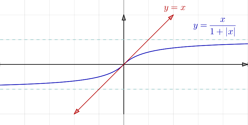
A titre indicatif, voici l’allure du graphe de $f,$ qui est symétrique par rapport à l’origine (puisque $f$ est impaire) et admet la première bissectrice pour tangente à l’origine. En outre, on peut signaler les deux asymptotes horizontales, d’équations $y=-1$ et $y=1.$

Remarque

On sait que la composée de deux applications dérivables est dérivable.

L’intérêt de cet exercice est de montrer que la dérivabilité d’une composée $g\circ f$ n’implique pas celle de $f$ et de $g.$ Sauriez-vous trouver un exemple de couple $\left(f,g\right)$ d’applications non dérivables tel que $g\circ f$ soit dérivable ?

Pour dévoiler une solution (parmi tant d’autres) … cliquer ici

Considérons la fonction indicatrice de $\mathbb{Q}$ :

$f:\mathbb{R}\rightarrow\mathbb{R},x\mapsto\left\{\begin{array}{cc}1 & \text{si }x\in\mathbb{Q}\\0 & \text{sinon}\end{array}\right.$

Il est bien connu que $f$ est discontinue en tout point (et qu’elle n’est donc dérivable nulle part). Pourtant $f\circ f$ est l’application constante $x\mapsto1$ qui est dérivable en tout point.

L’application $\left]-1,1\right[\rightarrow\mathbb{R},\thinspace x\mapsto{\displaystyle \frac{x}{\sqrt{1-x^{2}}}}$ est dérivable et donc $f$ aussi (composée d’applications dérivables). Pour tout $x\in\left]-1,1\right[$ :

$f'\left(x\right)=\frac{\sqrt{1-x^{2}}-x\:{\displaystyle \frac{-2x}{2\sqrt{1-x^{2}}}}}{1-x^{2}}\:\arctan'\left(\frac{x}{\sqrt{1-x^{2}}}\right)$

c’est-à-dire :

$f'\left(x\right)=\frac{1}{\left(1-x^{2}\right)^{3/2}}\:\frac{1}{1+{\displaystyle \frac{x^{2}}{1-x^{2}}}}$

soit finalement :

$f'\left(x\right)=\frac{1}{\sqrt{1-x^{2}}}$

Il s’ensuit l’existence d’un réel $A$ tel que :

$\forall x\in\left]-1,1\right[,\thinspace f\left(x\right)=\arcsin\left(x\right)+A$

et l’on voit, en évaluant en $x=0,$ que $A=0.$ En conclusion :

$\boxed{\forall x\in\left]-1,1\right[,\thinspace\arctan\left(\frac{x}{\sqrt{1-x^{2}}}\right)=\arcsin\left(x\right)}$

Remarque 1

Ce calcul intervient dans la preuve du lemme donnée à l’annexe 2 de cet article.

Remarque 2

Il existe une autre façon de traiter cet exercice, sans passer par un calcul de dérivée. Etant donné $x\in\left]-1,1\right[,$ on considère l’unique $\alpha\in\left]-\frac\pi2,\frac\pi2\right[$ tel que $x=\sin(\alpha)$ . On voit alors que :

$\arctan\left(\frac{x}{\sqrt{1-x^2}}\right)=\arctan\left(\tan(\alpha)\right)=\alpha=\arcsin(x)$

Supposons $f'$ impaire et montrons que $f$ est paire. Pour cela, posons pour tout $x\in\mathbb{R}$ :

$g\left(x\right)=f\left(x\right)-f\left(-x\right)$

Comme $f$ est dérivable, alors $g$ l’est aussi et, pour tout $x\in\mathbb{R}$ :

$g'\left(x\right)=f'\left(x\right)+f'\left(-x\right)=0$

donc $g$ est constante. Mais $g\left(0\right)=0$ et donc $g$ est identiquement nulle. Autrement dit $f$ est paire.

A présent, supposons $f'$ paire. On pourrait penser que cette hypothèse va entraîner l’imparité de $f,$ mais il n’en est rien (contre-exemple avec $f:x\mapsto x+1).$ Cependant, on peut adapter le calcul précédent et considérer l’application $h$ définie par :

$\forall x\in\mathbb{R},\thinspace h\left(x\right)=f\left(x\right)+f\left(-x\right)$

On voit que $h'$ est nulle, donc $h$ est constante et il existe $B\in\mathbb{R}$ tel que :

$\forall x\in\mathbb{R},\thinspace f\left(x\right)+f\left(-x\right)=B$

Ceci exprime, pour le graphe de $f,$ l’existence d’un centre de symétrie, à savoir le point $\left(0,{\displaystyle \frac{B}{2}}\right).$

Remarque

Toutefois, si $f'$ est paire et si de plus $f\left(0\right)=0,$ alors $f$ est impaire.

Supposons $f'\left(0\right)=0.$ Pour tout $n\in\mathbb{N}^{\star}$ et pour tout $x\in\mathbb{R}$ :

$\left(f^{n}\right)'\left(x\right)=\left(f^{n-1}\circ f\right)'\left(x\right)=\left(f^{n-1}\right)'\left(f\left(x\right)\right)\:\times\:f'\left(x\right)$

En particulier :

$\boxed{\left(f^{n}\right)'\left(0\right)=0}$

Supposons maintenant $f\left(0\right)=0$ et $f'\left(0\right)=1.$ Alors :

$\left(f^{n}\right)'\left(0\right)=\left(f^{n-1}\right)'\left(0\right)$

d’où (par une récurrence immédiate) $\left(f^{n}\right)'\left(0\right)=f'\left(0\right),$ soit :

$\boxed{\left(f^{n}\right)'\left(0\right)=1}$

D’après la formule de Leibniz (voir cet article). Pour tout $x\in\mathbb{R}$ et pour tout $n\in\mathbb{N}$ :

$f^{\left(n\right)}\left(x\right)=\sum_{k=0}^{n}\binom{n}{k}\exp^{\left(n-k\right)}\left(x\right)\sin^{\left(k\right)}\left(x\right)$

c’est-à-dire :

$f^{\left(n\right)}\left(x\right)=e^{x}\:\sum_{k=0}^{n}\binom{n}{k}\sin\left(x+\frac{k\pi}{2}\right)$

et donc, en particulier :

$f^{\left(n\right)}\left(0\right)=\sum_{k=0}^{n}\binom{n}{k}\sin\left(\frac{k\pi}{2}\right)$

Les termes d’indices pairs sont tous nuls et il reste donc :

$f^{\left(n\right)}\left(0\right)=\sum_{q=0}^{\left\lfloor \frac{n-1}{2}\right\rfloor }\binom{n}{2q+1}\sin\left(q\pi+\frac{\pi}{2}\right)=\sum_{q=0}^{\left\lfloor \frac{n-1}{2}\right\rfloor }\left(-1\right)^{q}\binom{n}{2q+1}$

On pourrait en rester là, mais il est tentant d’essayer de trouver une formule close pour cette dernière somme.

Voici l’astuce, qui fait un petit crochet par le champ complexe … On observe que :

$\sum_{k=0}^{n}\binom{n}{k}i^{k}=\left(1+i\right)^{n}=2^{n/2}\thinspace e^{in\pi/4}$

donc, en passant aux parties imaginaires :

$\sum_{q=0}^{\left\lfloor \frac{n-1}{2}\right\rfloor }\binom{n}{2q+1}\left(-1\right)^{q}=2^{n/2}\sin\left(\frac{n\pi}{4}\right)$

Finalement :

$\boxed{\forall n\in\mathbb{N},\thinspace f^{\left(n\right)}\left(0\right)=2^{n/2}\sin\left(\frac{n\pi}{4}\right)}$

Cela dit, puisqu’on s’est autorisé à passer par les complexes, autant y aller carrément ! On peut d’emblée observer que :

$\forall x\in\mathbb{R},\thinspace f\left(x\right)=\text{Im}\left(e^{\left(1+i\right)x}\right)$

Or, on sait que pour une fonction dérivable à valeurs complexes, la dérivée de la partie imaginaire est égale à la partie imaginaire de la dérivée … et donc :

$f^{\left(n\right)}\left(x\right)=\text{Im}\left(\left(1+i\right)^{n}\thinspace e^{\left(1+i\right)x}\right)$

d’où en particulier :

$f^{\left(n\right)}\left(0\right)=\text{Im}\left(\left(1+i\right)^{n}\right)$

et l’on retombe ainsi plus rapidement (et sans avoir besoin de la formule de Leibniz) sur le résultat encadré plus haut.

Lorsque $x$ est proche de 0, la variable d’intégration parcourt $\left[x,2x\right]$ donc se promène aussi au voisinage de $0$ et donc $e^{t}$ est voisin de 1. On peut donc conjecturer que $f\left(x\right)$ se comporte, lorsque $x$ tend vers 0, comme :

$\int_{x}^{2x}\frac{1}{t}\thinspace dt=\ln\left(2\right)$

Pour le prouver, on regarde la différence :

$f\left(x\right)-\ln\left(2\right)=\int_{x}^{2x}\frac{e^{t}-1}{t}\thinspace dt$

Cette quantité est positive (intégrale d’une fonction positive) et comme l’application $t\mapsto\frac{e^{t}-1}{t}$ admet une limite finie (égale à 1) en 0, elle est bornée sur $\left]0,1\right].$ Il existe $M>0$ tel que :

$\forall x\in\left]0,\frac{1}{2}\right],\thinspace0\leqslant f\left(x\right)-\ln\left(2\right)\leqslant Mx$

Cet encadrement prouve que :

$\boxed{\lim_{x\rightarrow0^{+}}f\left(x\right)=\ln\left(2\right)}$

On peut donc prolonger $f$ par continuité en $0$ en posant :

$\tilde{f}:\left[0,+\infty\right[\rightarrow\mathbb{R},\thinspace x\mapsto\left\{\begin{array}{cc}\ln\left(2\right) & \text{si }x=0\f\left(x\right) & \text{si }x>0\end{array}\right.$

On va maintenant s’intéresser à la dérivabilité de $\tilde{f}$ en 0. Posons pour tout $x>0$ :

$G\left(x\right)=\int_{1}^{x}\frac{e^{t}}{t}\thinspace dt$

$G$ est la primitive de $\left]0,+\infty\right[\rightarrow\mathbb{R},\thinspace{\displaystyle x\mapsto\frac{e^{x}}{x}}$ qui s’annule en 1. D’après la relation de Chasles, pour tout $x>0$ :

$f\left(x\right)=G\left(2x\right)-G\left(x\right)$

donc $f$ est dérivable sur $\left]0,+\infty\right[$ et pour tout $x>0$ :

$f'\left(x\right)=2\thinspace G'\left(2x\right)-G'\left(x\right)=\frac{e^{2x}-e^{x}}{x}$

En utilisant un développement limité au 1er ordre pour l’exponentielle, on voit que :

$\lim_{x\rightarrow0^{+}}f'\left(x\right)=1$

On en déduit, grâce au théorème de la limite de la dérivée, que $\tilde{f}$ est dérivable en $0$ et que :

$\boxed{\tilde{f}'\left(0\right)=1}$

Pour $x>0,$ l’intégrale

$\int_{0}^{+\infty}\frac{\sin\left(t\right)}{x+t}\thinspace dt$

est impropre pour la borne $+\infty.$ On voit avec une intégration par parties que, si $0<x<T$ alors :

$\begin{eqnarray*}\int_{0}^{T}\frac{\sin\left(t\right)}{x+t}\thinspace dt & = & \left[\frac{-\cos\left(t\right)}{x+t}\right]_{t=0}^{T}-\int_{0}^{T}\frac{\cos\left(t\right)}{\left(x+t\right)^{2}}\thinspace dt\\& = & \frac{1}{x}-\frac{\cos\left(T\right)}{x+T}-\int_{0}^{T}\frac{\cos\left(t\right)}{\left(x+t\right)^{2}}\thinspace dt \end{eqnarray*}$

Comme l’intégrale $\int_{0}^{+\infty}\frac{\cos\left(t\right)}{\left(x+t\right)^{2}}\thinspace dt$ est absolument convergente, elle est convergente et donc l’intégrale partielle $\int_{0}^{T}\frac{\sin\left(t\right)}{x+t}\thinspace dt$ admet, lorsque $T$ tend vers $+\infty,$ une limite finie à savoir :

$\lim_{T\rightarrow+\infty}\int_{0}^{T}\frac{\sin\left(t\right)}{x+t}\thinspace dt=\frac{1}{x}-\int_{0}^{+\infty}\frac{\cos\left(t\right)}{\left(x+t\right)^{2}}\thinspace dt$

Bref, $f$ est bien définie. Ensuite, le changement de variable $s=x+t$ donne :

$f\left(x\right)=\int_{x}^{+\infty}\frac{\sin\left(s-x\right)}{s}\thinspace ds$

et donc, d’après la formule d’addition pour le sinus :

$f\left(x\right)=\cos\left(x\right)\int_{x}^{+\infty}\frac{\sin\left(s\right)}{s}\thinspace ds-\sin\left(x\right)\int_{x}^{+\infty}\frac{\cos\left(s\right)}{s}\thinspace ds$

Pour alléger un peu l’écriture, notons :

$C\left(x\right)=\int_{x}^{+\infty}\frac{\cos\left(s\right)}{s}\thinspace ds\qquad\text{et}\qquad S\left(x\right)=\int_{x}^{+\infty}\frac{\sin\left(s\right)}{s}\thinspace ds$

de sorte que :

$f\left(x\right)=\cos\left(x\right)S\left(x\right)-\sin\left(x\right)C\left(x\right)$

A partir de là, il est facile de dériver :

$f'\left(x\right)=-\sin\left(x\right)S\left(x\right)-\cos\left(x\right)C\left(x\right)+\cos\left(x\right)S'\left(x\right)-\sin\left(x\right)C'\left(x\right)$

Or :

$C'\left(x\right)=-\frac{\cos\left(x\right)}{x}\qquad\text{et}\qquad S'\left(x\right)=-\frac{\sin\left(x\right)}{x}$

et donc :

$f'\left(x\right)=-\sin\left(x\right)S\left(x\right)-\cos\left(x\right)C\left(x\right)$

On dérive encore un coup :

$\begin{eqnarray*} f''\left(x\right) & = & -\cos\left(x\right)S\left(x\right)+\sin\left(x\right)C\left(x\right)-\sin\left(x\right)S'\left(x\right)-\cos\left(x\right)C'\left(x\right)\\ & = & -f\left(x\right)+\frac{\sin^{2}\left(x\right)+\cos^{2}\left(x\right)}{x}\\ & = & -f\left(x\right)+\frac{1}{x} \end{eqnarray*}$

En définitive, on a prouvé que :

$\boxed{\forall x>0,\thinspace f''\left(x\right)+f\left(x\right)=\frac{1}{x}}$

Comme $\deg\left(P\right)$ est impair, alors $P$ possède (au moins) une racine réelle $a.$ L’hypothèse impose :

$\forall n\in\mathbb{N},\thinspace f^{\left(n\right)}\left(a\right)=0$

Pour tout $x\in\mathbb{R}$ et pour tout $n\in\mathbb{N},$ la formule de Taylor avec reste intégral donne :

$f\left(x\right)=\int_{a}^{x}\frac{\left(x-t\right)^{n}}{n!}f^{\left(n+1\right)}\left(t\right)\thinspace dt$

et donc :

( $\star$ ) $\left|f\left(x\right)\right|\leqslant\frac{\left|x-a\right|^{n+1}}{n!}\sup\left\{\left|P\left(t\right)\right|;\thinspace t\in\left[a,x\right]\right\}$

Or, on sait que :

$\forall\lambda\in\mathbb{R},\thinspace\lim_{n\rightarrow\infty}\frac{\lambda^{n}}{n!}=0$

En passant à la limite (pour $x$ fixé et en faisant tendre $n$ vers $+\infty)$ dans $\left(\star\right),$ on conclut que $f$ est l’application nulle.

On peut traiter cette question en combinant deux outils : d’une part, le lemme de Rolle et, d’autre part, le petit artifice technique suivant …

Si l’on pose, pour tout $t\in\mathbb{R}$ :

$h\left(t\right)=f\left(t\right)\thinspace e^{\alpha t}$

alors :

$h'\left(t\right)=\left(f'\left(t\right)+\alpha\thinspace f\left(t\right)\right)\thinspace e^{\alpha t}=g\left(t\right)\thinspace e^{\alpha t}$

ce qui montre que les zéros de $g$ sont ceux de $h'.$

Supposons $n\geqslant2.$ Par hypothèse, il existe des réels $t_{1}<\cdots<t_{n}$ tels que, pour tout $i\in\left\llbracket 1,n\right\rrbracket ,$ $f\left(t_{i}\right)=0$ et donc $h\left(t_{i}\right)=0.$ En appliquant le lemme de Rolle à $h$ sur chacun des segments $\left[t_{i},t_{i+1}\right],$ on voit qu’il existe des réels $c_{1}<\cdots<c_{n-1}$ tels que :

$\forall i\in\left\llbracket 1,n-1\right\rrbracket ,\thinspace h'\left(c_{i}\right)=0$

et donc :

$\forall i\in\left\llbracket 1,n-1\right\rrbracket ,\thinspace g\left(c_{i}\right)=0$

Il reste à montrer l’existence d'(au moins) un $n-$ ème zéro pour $g.$ Ceci va découler du résultat suivant :

Lemme de Rolle étendu aux intervalles non bornés

Soit $\varphi:\left[a,+\infty\right[\rightarrow\mathbb{R}$ une application continue. On suppose que $\varphi$ est dérivable sur $\left]a,+\infty\right[$ et que :

$\lim_{t\rightarrow+\infty}\varphi\left(t\right)=\varphi\left(a\right)$

Alors il existe $c\in\left]a,+\infty\right[$ vérifiant $\varphi'\left(c\right)=0.$

Si $\alpha<0$ alors vu que $f$ est bornée, on voit que $h$ est bornée sur $\left[t_{n},+\infty\right[$ et donc, en appliquant ce lemme à $h$ sur cet intervalle, on met en évidence un réel $c_n$ tel que $c_n>t_n$ et $h'\left(c_n\right)=0,$ d’où $g\left(c_n\right)=0.$

De même, si $\alpha>0,$ on procède de même, mais sur l’intervalle $\left]-\infty,t_{1}\right]$ , ce qui donne l’existence d’un réel $c_0<c_1$ tel que $g(c_0)=0$ .

Bref, dans tous les cas, on constate que $g$ s’annule (au moins) $n$ fois.

Si un point n’est pas clair ou vous paraît insuffisamment détaillé, n’hésitez pas à poster un commentaire ou à me joindre via le formulaire de contact.

Partager cet article